סקלרים, פונקציות ומשפטי התנייה
תרגיל בית 2
import math

# Updated find_max_number to handle all cases, including ties and floats
def find_max_number(num1, num2, num3):
    return max(num1, num2, num3)

# Calculates the mean of three numbers
def find_mean(num1, num2, num3):
    return (num1 + num2 + num3) / 3

# Calculates the mean and standard deviation of three numbers
def find_mean_std(num1, num2, num3):
    mean = find_mean(num1, num2, num3)
    variance = ((num1 - mean) ** 2 + (num2 - mean) ** 2 + (num3 - mean) ** 2) / 3
    std = math.sqrt(variance)
    return mean, std
הנוסחה לחישוב סטיית תקן היא:
\[\sigma = \sqrt{\frac{\sum_{i=1}^{n} (x_i - \mu)^2}{n}}\]כאשר $\sigma$ היא סטיית התקן, $x_i$ הוא ערך ספציפי בסדרה, $\mu$ היא הערך הממוצע של הסדרה, ו$n$ הוא מספר הערכים בסדרה.
שימוש נפוץ בסטיית התקן שמופיע בנושא של עיבוד מידע וגרפים, הוא ניקוי מידע חריג (outliers) מהנתונים. התהליך הזה מחשב עד כמה כל נתון רחוק מהערך הממוצע של הנתונים, ומסיר את הנתונים שרחוקים מדי מהערך הממוצע - בדרך כלל נתונים שרחוקים מהערך הממוצע ביותר משתי סטיות תקן (בדוגמת הפינגווין דווא רחוקים מסטיית תקן אחת). להרחבה ראו דוגמת הפינגווינים בגרסה אינטראקטיבית.
אוספים, לולאות
איך ניתן לקבל את מספר האלמנטים ברשימה
my_list
my_list = [1, 2, 3, 4, 5]
len(my_list)my_list.length()- not a method for listsmy_list.size()- not a method for listsmy_list.count()- counts how many times an element appears in the list
כיצד ניתן להוריד את הסימון
n\לשורה חדשה מהמחרוזת הבאה?
my_string = "TAG\tStp\tO\tStop\n"
my_string.split()- will split the string into a list of strings separated by whitespace (‘\t’, ‘\n’, ‘ ‘).my_string.strip()- will remove leading and trailing whitespace, including ‘\n’.my_string.replace("\n", "")- will replace all occurrences of ‘\n’ with an empty string.strip(my_string, "\n")- not a valid function in Python.my_string.split("\n")- will split the string into a list of strings separated by ‘\n’, in this case, it will return the original string and an empty string:['TAG\tStp\tO\tStop', ''].
my_string = "TAG\tStp\tO\tStop\n"

print(my_string)
TAG	Stp	O	Stop

print(my_string.strip())
TAG	Stp	O	Stop
print(my_string)
TAG	Stp	O	Stop

print(my_string.split())
['TAG', 'Stp', 'O', 'Stop']
print(my_string.split("\n"))
['TAG\tStp\tO\tStop', '']
print(my_string.replace("\n", ""))
TAG	Stp	O	Stop
print(my_string)
TAG	Stp	O	Stop
תרגיל בית 3 - רשימות ולולאות
def move(my_list, direction):

    # Finds the index of the one in the list
    index_of_one = my_list.index(1)

    # handle edge cases
    if index_of_one == 0 and direction == 'left':
        return my_list
    elif index_of_one == len(my_list) - 1 and direction == 'right':
        return my_list

    # Move the one to the left or to the right
    if direction == 'right':
        my_list[index_of_one] = 0
        my_list[index_of_one + 1] = 1

    elif direction == 'left':
        my_list[index_of_one] = 0
        my_list[index_of_one - 1] = 1

    return my_list
def approximate_pi(n_terms):
    """
    Approximate pi using the Leibniz series.
    """
    pi = 0
    for i in range(n_terms):
        pi += (-1) ** i / (2 * i + 1)
    return 4 * pi # Multiply by 4 to get pi
למדנו בשיעור על אוספים למעשה מחרוזות (
Strings) הן גם אוספים - של תווים. המחרוזות הן:immutable,orderו -not-unique. לפיכך, סמנו את הפעולה או הפעולות המותרות על מחרוזות. ניתן לסמן יותר מתשובה אחת.
- שינוי - לא ניתן כי הן
immutable - הוספה - לא ניתן כי הן
immutable, אבל בעיקרון ניתן לחבר אותן לתוך מחרוזת חדשה - הורדה / מחיקת איבר - לא ניתן כי הן
immutable - קריאה
תרגיל בית 4 - מחרוזות ולולאות
def split_before_each_uppercases(formula):
    """
    Split a string before each uppercase letter.
    """
    result = []
    temp = ""

    for char in formula:
        if char.isupper() and temp:
            result.append(temp)
            temp = char
        else:
            temp += char

    if temp:
        result.append(temp)

    return result
def split_at_first_digit(formula):
    """
    Split a string into a tuple of (non-digit part, numeric part).
    If no digits are found, return the original string and 1.

    Args:
    formula (str): The input string to be split.

    Returns:
    tuple: A tuple with the non-digit part as a string and the digit part as an integer.
    """
    for i, c in enumerate(formula):
        if c.isdigit():  # Find the first digit
            return formula[:i], int(formula[i:])
    return formula, 1  # Default to returning the formula and 1 if no digit is found
סדר וארגון
תרגיל בית 5 - מילונים ומודולים
def split_before_each_uppercases(formula):
    """
    Split a string before each uppercase letter.
    """
    result = []
    temp = ""

    for char in formula:
        if char.isupper() and temp:
            result.append(temp)
            temp = char
        else:
            temp += char

    if temp:
        result.append(temp)

    return result

def split_at_number(formula):
    """
    Split a string into a tuple of (non-number part, numeric part).
    If no numbers are found, return the original string and 1.

    Args:
    formula (str): The input string to be split.

    Returns:
    tuple: A tuple with the non-number part as a string and the number part as an integer.
    """
    for i, c in enumerate(formula):
        if c.isdigit():  # Find the first digit
            return formula[:i], int(formula[i:])
    return formula, 1  # Default to returning the formula and 1 if no digit is found


def split_at_first_digit(formula):
    """
    Split a string into a tuple of (non-digit part, numeric part).
    If no digits are found, return the original string and 1.

    Args:
    formula (str): The input string to be split.

    Returns:
    tuple: A tuple with the non-digit part as a string and the digit part as an integer.
    """
    for i, c in enumerate(formula):
        if c.isdigit():  # Find the first digit
            return formula[:i], int(formula[i:])
    return formula, 1  # Default to returning the formula and 1 if no digit is found
def count_atoms_in_molecule(molecular_formula):
    """Takes a molecular formula (string) and returns a dictionary of atom counts.
    Example: 'H2O' → {'H': 2, 'O': 1}"""

    def split_by_capitals(formula):
        """Split a string before each uppercase letter."""
        result = []
        temp = ""

        for char in formula:
            if char.isupper() and temp:
                result.append(temp)
                temp = char
            else:
                temp += char

        if temp:
            result.append(temp)

        return result
    # Step 1: Initialize an empty dictionary to store atom counts
    atom_counts = {}

    for atom in split_by_capitals(molecular_formula):
        atom_name, atom_count = split_at_number(atom)

        # Step 2: Update the dictionary with the atom count
        if atom_name in atom_counts:
            atom_counts[atom_name] += int(atom_count)
        else:
            atom_counts[atom_name] = int(atom_count)

    # Step 3: Return the completed dictionary
    return atom_counts


def parse_chemical_reaction(reaction_equation):
    """Takes a reaction equation (string) and returns reactants and products as lists.
    Example: 'H2 + O2 -> H2O' → (['H2', 'O2'], ['H2O'])"""
    reaction_equation = reaction_equation.replace(" ", "")  # Remove spaces for easier parsing
    reactants, products = reaction_equation.split("->")
    return reactants.split("+"), products.split("+")

def count_atoms_in_reaction(molecules_list):
    """Takes a list of molecular formulas and returns a list of atom count dictionaries.
    Example: ['H2', 'O2'] → [{'H': 2}, {'O': 2}]"""
    molecules_atoms_count = []
    for molecule in molecules_list:
        molecules_atoms_count.append(count_atoms_in_molecule(molecule))
    return molecules_atoms_count
קובצי נתונים
איזה מודול אחראי לקריאת קוד ה-
HTMLמהאתר?
import requests
from bs4 import BeautifulSoup

url = 'https://MedInTzfat.com'
response = requests.get(url)
soup = BeautifulSoup(response.text, 'html.parser')
requests
תרגיל בית 6
def create_codon_dict(filename):
    codon_dict = {}
    with open(filename, 'r') as file:
        for line in file:
            codon, amino_acid, single_letter, full_name = line.split()
            codon_dict[codon] = single_letter
    return codon_dict
הרשאות בקבצים
הערה על הרשאות (permissions) לקובץ:
| סוג הרשאה | תיאור |
|---|---|
r | קריאה |
w | כתיבה |
x | יצירה |
a | הוספה |
t | טקסט |
b | בינארי |
מתוך התיעוד הרשמי:
| Mode | Description |
|---|---|
r | Open a file for reading. (default) |
w | Open a file for writing. Creates a new file if it does not exist or truncates the file if it exists. |
x | Open a file for exclusive creation. If the file already exists, the operation fails. |
a | Open for appending at the end of the file without truncating it. Creates a new file if it does not exist. |
t | Open in text mode. (default) |
b | Open in binary mode. |
+ | Open a file for updating (reading and writing). |
גרפים
matplotlib
fig, axs = plt.subplots(1,2, figsize=(10,5))
axs הוא מערך (numpy array) של אובייקטים מסוג Axes, שכל אחד מהם מייצג גרף בודד בתוך ה-Figure. כאשר plt.subplots(rows, cols) מחזיר מספר תת-גרפים (subplots), axs מכיל את הצירים של כל אחד מהם. אם יש יותר מעמודה אחת, axs הוא מערך של צירים בגודל (rows, cols). אם יש רק עמודה אחת או רק שורה אחת, axs יהיה מערך חד-ממדי.
import matplotlib.pyplot as plt

fig, axs = plt.subplots(1, 2, figsize=(10, 5))

print(type(axs))        # <class 'numpy.ndarray'>
print(axs.shape)        # (2,)
print(type(axs[0]))     # <class 'matplotlib.axes._subplots.AxesSubplot'>
פינגווינים
import pandas as pd
url_csv = "https://raw.githubusercontent.com/mwaskom/seaborn-data/refs/heads/master/penguins.csv"
data = pd.read_csv(url_csv)
print(data.head(5))
"""
(.venv) dorpascal@Mac-mini tzfat % /usr/local/bin/python3.11 /U
sers/dorpascal/projects.nosync/tzfat/python/penguins.py
species island ... body_mass_g sex
0 Adelie Torgersen ... 3750.0 MALE
1 Adelie Torgersen ... 3800.0 FEMALE
2 Adelie Torgersen ... 3250.0 FEMALE
3 Adelie Torgersen ... NaN NaN
4 Adelie Torgersen ... 3450.0 FEMALE
"""
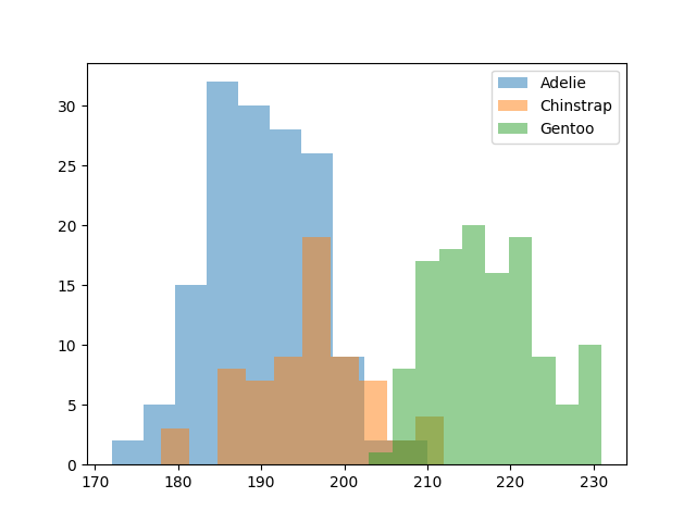
import matplotlib.pyplot as plt
groupd = data.groupby('species')
for species, species_data in groupd:
plt.hist(species_data['flipper_length_mm'], label=species, alpha=0.5)
plt.legend()
plt.show()
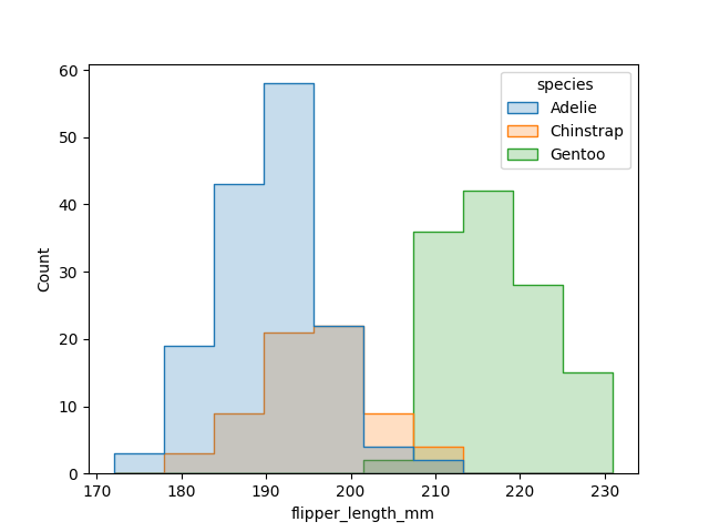
שימוש ב-seaborn
import pandas as pd

url_csv = "https://raw.githubusercontent.com/mwaskom/seaborn-data/refs/heads/master/penguins.csv"

data = pd.read_csv(url_csv)
print(data.head(5))

"""
(.venv) dorpascal@Mac-mini tzfat % /usr/local/bin/python3.11 /U
sers/dorpascal/projects.nosync/tzfat/python/penguins.py
  species     island  ...  body_mass_g     sex
0  Adelie  Torgersen  ...       3750.0    MALE
1  Adelie  Torgersen  ...       3800.0  FEMALE
2  Adelie  Torgersen  ...       3250.0  FEMALE
3  Adelie  Torgersen  ...          NaN     NaN
4  Adelie  Torgersen  ...       3450.0  FEMALE
"""


import seaborn as sns

sns.histplot(data, x='flipper_length_mm', hue='species', element='step')

import matplotlib.pyplot as plt

plt.show()
שאלון בית 7
סיכום התשובות הנכונות:
-
הוספת כותרת בעזרת
pltנעשית באמצעות הפונקציהplt.title("My Title")ואילו הוספת כותרת לתת־גרף (subplot) בעזרת אובייקט
axנעשית באמצעותax.set_title("My Title") -
הפרמטר
binsבפונקציהplt.histמגדיר את מספר העמודות (intervals) בהיסטוגרמה. -
df["A"](ב־DataFrame שנקראdf) מחזיר את כל נתוני העמודה ששמה “A”. -
ארגומנט חובה לפונקציה
plt.savefigהוא מסלול ושם הקובץ שאליו אנו שומרים את הגרף, לדוגמה:plt.savefig("path/to/figure.png")
תרגיל בית 7
# Import libraries
import matplotlib.pyplot as plt
import seaborn as sns
from sklearn.datasets import fetch_openml
# Step 1: Select a Dataset
data = fetch_openml(name='iris', version=1, as_frame=True)
# Step 2: Inspect the Data
print(data.DESCR)
df = data.frame
print(df.head())
print("Sample data:")
print(df.sample(5))
print("Summary statistics:")
print(df.describe())
print("Data types:")
print(df.dtypes)
# Step 3: Select Features
features = list(df.columns)
print("Available features:", features)
selected_features = [features[0], features[2]]
print("Selected features: ", selected_features)
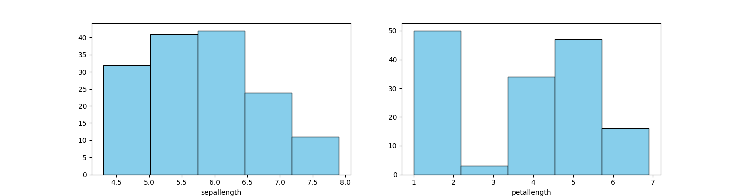
# Step 4: Make Histogram Plots
fig, axs = plt.subplots(1, len(selected_features), figsize=(20, 3))
for ax, f in zip(axs, selected_features):
ax.hist(df[f], bins=5, color='skyblue', edgecolor='black')
ax.set_xlabel(f)
plt.show()
# Step 5: Test Correlation with Scatter Plots
reference_feature = selected_features[1]
y = df[reference_feature]
fig, axs = plt.subplots(1, len(features), figsize=(20, 3))
for ax, f in zip(axs, features):
ax.scatter(df[f], y)
ax.set_xlabel(f)
plt.show()
# Step 6: Save a Selected Correlation Plot
reference_feature = selected_features[0]
comparison_feature = selected_features[1]
plt.figure(figsize=(8, 6))
plt.scatter(df[reference_feature], df[comparison_feature], alpha=0.6)
plt.xlabel(reference_feature)
plt.ylabel(comparison_feature)
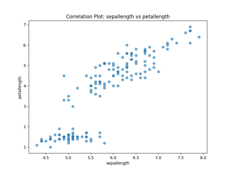
plt.title("Correlation Plot: {} vs {}".format(reference_feature, comparison_feature))
# Save the plot
plt.savefig('correlation_plot.png')
plt.show()
Analysis
Dataset Overview
For this assignment, I chose the Iris dataset. This dataset contains 150 samples of iris flowers, each with four features (sepal length, sepal width, petal length, and petal width) and a target label (species).
The dataset includes the following key features:
- Feature 1: Sepal Length (cm)
- Feature 2: Sepal Width (cm)
- Feature 3: Petal Length (cm)
- Feature 4: Petal Width (cm)
- Target: Species (setosa, versicolor, virginica)
- Classes: 3
- Data Points: 150
Steps Followed
1. Data Exploration
- Structure and Summary:
- The dataset consists of 150 rows and 5 columns.
- Data Types:
- Features include float values, and the target is a categorical variable.
- Random Sample:
- A quick look at 5 random rows helped ensure data validity.
Analysis output:
(.venv) dorpascal@MacBook-Air-4 ps7-visualization-Dor-sketch % python3 ./main.py
**Author**: R.A. Fisher
**Source**: [UCI](https://archive.ics.uci.edu/ml/datasets/Iris) - 1936 - Donated by Michael Marshall
**Please cite**:

**Iris Plants Database**
This is perhaps the best known database to be found in the pattern recognition literature.  Fisher's paper is a classic in the field and is referenced frequently to this day.  (See Duda & Hart, for example.)  The data set contains 3 classes of 50 instances each, where each class refers to a type of iris plant.  One class is     linearly separable from the other 2; the latter are NOT linearly separable from each other.

Predicted attribute: class of iris plant.
This is an exceedingly simple domain.

### Attribute Information:
    1. sepal length in cm
    2. sepal width in cm
    3. petal length in cm
    4. petal width in cm
    5. class:
       -- Iris Setosa
       -- Iris Versicolour
       -- Iris Virginica

Downloaded from openml.org.
   sepallength  sepalwidth  petallength  petalwidth        class
0          5.1         3.5          1.4         0.2  Iris-setosa
1          4.9         3.0          1.4         0.2  Iris-setosa
2          4.7         3.2          1.3         0.2  Iris-setosa
3          4.6         3.1          1.5         0.2  Iris-setosa
4          5.0         3.6          1.4         0.2  Iris-setosa
Sample data:
     sepallength  sepalwidth  petallength  petalwidth            class
41           4.5         2.3          1.3         0.3      Iris-setosa
50           7.0         3.2          4.7         1.4  Iris-versicolor
133          6.3         2.8          5.1         1.5   Iris-virginica
93           5.0         2.3          3.3         1.0  Iris-versicolor
144          6.7         3.3          5.7         2.5   Iris-virginica
Summary statistics:
       sepallength  sepalwidth  petallength  petalwidth
count   150.000000  150.000000   150.000000  150.000000
mean      5.843333    3.054000     3.758667    1.198667
std       0.828066    0.433594     1.764420    0.763161
min       4.300000    2.000000     1.000000    0.100000
25%       5.100000    2.800000     1.600000    0.300000
50%       5.800000    3.000000     4.350000    1.300000
75%       6.400000    3.300000     5.100000    1.800000
max       7.900000    4.400000     6.900000    2.500000
Data types:
sepallength     float64
sepalwidth      float64
petallength     float64
petalwidth      float64
class          category
dtype: object
Available features: ['sepallength', 'sepalwidth', 'petallength', 'petalwidth', 'class']
Selected features:  ['sepallength', 'petallength']
2024-12-15 09:53:53.818 Python[48964:5660928] +[IMKClient subclass]: chose IMKClient_Modern
2024-12-15 09:53:53.819 Python[48964:5660928] +[IMKInputSession subclass]: chose IMKInputSession_Modern
(.venv) dorpascal@MacBook-Air-4 ps7-visualization-Dor-sketch %
2. Selected Features
From the dataset, I selected the following features for detailed analysis:
- Feature A: Sepal Length (cm)
- Feature B: Petal Length (cm)
3. Visualization
Histograms
Scatter Plots
Scatter plots were generated to explore correlations between the selected features:
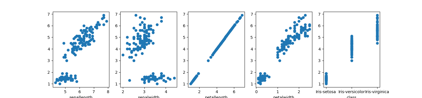
- First Plot: Sepal Length vs Petal Length (cm)
- This plot ahows a positive linear relationship between Sepal Length and Petal Length. Aka, as Sepal Length increases, Petal Length also increases.
- Second Plot: Sepal Width vs Petal Length (cm)
- This plot shows a weak correlation between Sepal Width and Petal Length.
- The data points are scattered, indicating no clear relationship between the two features.
- Third Plot: Petal length vs Petal length (cm)
- This plot shows a strong positive linear relationship since we compare the same feature.
- Forth Plot: Petal width vs Petal length (cm)
- This plot shows a strong positive linear relationship between Petal Width and Petal Length.
- Fifth Plot: Class vs Petal length (cm)
- This plot shows a clear separation of the classes based on Petal Length.
- Iris-setosa has the smallest Petal Length, while Iris-virginica has the largest.
- Iris-versicolor falls in between the other two classes.
- This indicates that Petal Length is a good feature for classifying the iris species.
Key Insights
Correlation Plot Analysis
I chose the scatter plot for sepallength vs peta length for further analysis because:
- It showed a strong positive linear relationship.
- This suggests that Sepal Length is a good predictor for Petal Length.
- The plot was saved as
correlation_plot.png.
Patterns Observed
- Positive Correlation:
- Sepal Length and Petal Length showed a strong positive correlation.
- As Sepal Length increased, Petal Length also increased.
- This indicates a linear relationship between the two features.
- The scatter plot showed a clear pattern of data points aligned in a positive direction.
- This suggests that Sepal Length can be a good predictor for Petal Length.
Conclusion
This analysis highlights:
- The importance of selecting relevant features for analysis.
- The significance of visualizations in understanding data relationships.
- The value of correlation analysis in identifying patterns and trends.
- The potential of certain features as predictors for target variables.
- The need for further exploration to gain deeper insights into the dataset.
By following these steps, we can gain valuable insights from the data and make informed decisions based on the analysis.
עיבוד מידע
שאלון 8
עבור הטבלה df הבאה:
| Caregory | Value | |
|---|---|---|
| 0 | A | 10 |
| 1 | B | 20 |
| 2 | A | 30 |
| 3 | B | 40 |
מה יהיה הפלט של הקוד הבא:
df.groupby('Category').max()
מה יהיה הפלט של הקוד הבא:
df.groupby('Category').sum()
למידת מכונה
עבור מערכת המקבלת נתונים מספריים רציפים וצריך לחזות נתון מספרי רציף אחר. באיזה מודל נרצה להשתמש? ניתן לסמן יותר מתשובה אחת.
Linear regressionK nearest neighborsDecision treeK-means
איזה מודל רגיש לסקלה (לכיול) של המספרים שהוא מקבל כקלט? ניתן לסמן יותר מתשובה אחת.
Decision treeK nearest neighborsLinear regressionK-means
הסבר מפורט
כאשר שואלים על “רגישות לסקלה” (Scale Sensitivity), מתכוונים למודל שבו שינוי ביחידות או בטווח של התכונות (Features) עלול להשפיע משמעותית על הביצועים או על תוצאות החיזוי. במילים אחרות, אם נרחיב או נכווץ את הסקאלה של אחת התכונות, האם המודל “יתבלבל” או יניב תוצאות שונות בצורה מהותית?
1. Decision Tree (עץ החלטה)
- מודל זה בוחר פיצולים (Splits) לפי מידע אנטרופי או מידע גייני (Information Gain), ולא על סמך מרחקים בין נקודות.
- בשל כך, בדרך כלל לא חייבים לבצע נורמליזציה או סטנדרטיזציה של התכונות. עץ ההחלטה מחלק את הנתונים ע”פ תנאים בוליאניים (כמו
x < some_value), ולכן סדר הגודל שלxפחות קריטי. - לכן, עץ החלטה אינו רגיש לסקלה.
2. K-Nearest Neighbors (KNN)
- מודל המבוסס כולו על חישוב מרחק (לרוב מרחק אוקלידי או מרחק מנהטן) בין דגימות.
- אם סקאלת התכונות שונה, תכונה בעלת ערכים גדולים תקבל משקל יתר בחישוב המרחק, ותשפיע על הדירוג (הקרובים ביותר).
- לכן, KNN רגיש מאוד לסקלה – מומלץ לבצע סטנדרטיזציה/נורמליזציה לפני שימוש במודל זה.
3. Linear Regression (רגרסיה לינארית)
- רגרסיה לינארית בגרסה הבסיסית שלה (בלי רגולריזציה) לא “תשתגע” אם נשנה את סקאלת התכונות, משום שהפתרון האנליטי פשוט יתאים את משקליו (המקדם $\beta$ גדל או קטן בהתאם).
- ברמת הביצועים (ללא רגולריזציה) אין לכך השפעה ישירה על דיוק המודל, אם כי מבחינה מספרית/חישובית זה יכול להשפיע על קצב התכנסות בגישות כמו Gradient Descent.
- בנוסף, אם מכניסים רגולריזציה (למשל Ridge או Lasso), אז סקיילינג נעשה חשוב כדי לא להטות את משקלי התכונות.
- ועדיין, בהשוואה למודלים מבוססי מרחק, רגרסיה לינארית נחשבת פחות “רגישה” לסקאלות – אפשר בהחלט לסמן אותה כלא-רגישה בהקשר הספציפי של השאלה הזו.
4. K-Means
- אלגוריתם של אשכולות (Clustering) המחשב את מרכזי הקלאסטרים (Centroids) באמצעות ממוצע מרחבי, ומקצה נקודות לפי המרחק שלהן מהמרכזים הללו.
- בדומה ל-KNN, גם כאן מרחק הוא כלי מרכזי – על כן, אם לא מנרמלים/מסטנדרטים, תכונות בקנה מידה גדול “ישתלטו” על המרחק.
- מסקנה: K-Means רגיש לסקאלה.
אנחנו מבצעים חלוקה של הנתונים לקבוצת אימון ולקבוצת בדיקה. מדוע קבוצת הנתונים של הבדיקה חשובה?
- על מנת לקבל הערכה מספרים לאיכות המודל.
- על מנת שנוכל לבצע חיזוי.
- על-מנת שנוכל להמשיך ולאמן את המודל בעתיד.
- היא נועדה לנקות נתונים בעייתים.
הסבר: קבוצת הבדיקה (Test set) משמשת לבדיקת איכות המודל שנבנה על ידי קבוצת האימון (Training set). על ידי השוואת התוצאות של המודל על קבוצת הבדיקה לתוצאות המקוריות, ניתן להעריך את יכולת המודל להתמודד עם נתונים חדשים ולבצע חיזויים נכונים.
הכרנו את הגדלים הבאים:
- Acc - Accuracy
- TP - True positive
- FP - False positive
- TN- True negative
- FN - false negative
מצאו את הקשר הנכון בין הגדלים.
Acc = (TP + TN)/(FN + FP)Acc = (TP + TN)Acc = (TP)/(TP + FP)Acc = (TP + TN)/(TP + TN + FN + FP)
שאלון בית 9 - למידת מכונה
פירוט וקישור למאמר במאמר “Suitability of dysphonia measurements for telemonitoring of Parkinson’s disease” (Little ואח׳), החוקרים בדקו אילו מדדים אקוסטיים (Features) מאפשרים להבחין בצורה מיטבית בין אנשים בריאים לבין חולי פרקינסון על סמך דגימות דיבור (sustained phonations).
שאלה 1: מהם ארבעת המדדים המובילים (למשימת הקִטלוג)?
מן המאמר עולה בבירור (ראו טבלה 3 וסיכום התוצאות במאמר) כי שילוב ארבעת המדדים הבאים הוביל לאחוזי הסיווג הגבוהים ביותר (כ‑91.4% הצלחה):
- PPE – Pitch Period Entropy
- DFA – Detrended Fluctuation Analysis
- RPDE – Recurrence Period Density Entropy
- HNR – Harmonics-to-Noise Ratio
ציטוט רלוונטי מהמאמר (טבלה 3):
“When taken in combination, HNR, RPDE, DFA and PPE obtains best overall classification performance of 91.4%, using an SVM classifier.”
שאלה 2: מהו המדד PPE המוצג במאמר?
המאמר מציג את PPE (Pitch Period Entropy) כמדד חדש המודד את מידת האי‑סדירות (entropy) בהפרשים היחסיים של ה‑Pitch (מחזורי הקול) לאחר סינון ושקלול על סקאלה לוגריתמית (סקאלת semitone).
התשובה הנכונה: Pitch Period Entropy
שאלה 3: מהו מודל הלמידה (Machine/Deep Learning) שנבחר?
החוקרים השתמשו במספר אלגוריתמי סיווג להשוואה, אך מודל ה‑SVM (Support Vector Machine) עם גרעין (Kernel) רדיאלי הראה את התוצאות הטובות ביותר לסיווג בין חולי פרקינסון לבין אנשים בריאים.
התשובה הנכונה: SVM
הסבר קצר על הבחירה ב‑SVM
החוקרים מדגישים שהחלטה זו התקבלה לאחר ניסוי של כל קומבינציית פיצ׳רים (Features) אפשרית מתוך 10 מדדים לא-מתואמים. האלגוריתם שסיפק את ביצועי הסיווג הטובים ביותר בהקשר של המשימה (טלמוניטורינג של פרקינסון) היה SVM עם Radial Basis Function Kernel, מבחינת אחוזי הצלחה כלליים, אחוזי True Positive (חולי פרקינסון שסווגו נכון) ואחוזי True Negative (בריאים שסווגו נכון).
למה PPE, DFA, RPDE ו‑HNR?
- PPE מודד תנודתיות חריגה בגובה הצליל (Pitch) אחרי הסרת תנודות “בריאות” רגילות.
- DFA (Detrended Fluctuation Analysis) מאתר את רמת ה-“self-similarity” בנוכחות רעש נשיפתי (Turbulent noise) המתגבר במצב דיספוניה.
- RPDE (Recurrence Period Density Entropy) בודק עד כמה האות קבוע וחוזר על עצמו תקופתית. אצל חולי פרקינסון יש פחות חזרתיות סדירה במחזורי הקול.
- HNR (Harmonics-to-Noise Ratio) הוא מדד מסורתי הלוכד את היחס בין הרכיב ההרמוני (קול צלול) לבין הרכיב הרועש בדגימה.
השילוב של שלושת המדדים הלא-מסורתיים (PPE, DFA, RPDE) יחד עם HNR המסורתי נתן, בפועל, את התוצאות הטובות ביותר.
ציטוט מסכם מהמאמר
“In conclusion, we find that non-standard methods in combination with traditional harmonics-to-noise ratios are best able to separate healthy from PD subjects. The selected non-standard methods are robust to many uncontrollable variations in acoustic environment and individual subjects, and are thus well-suited to telemonitoring applications.”
תרגיל בית 8
import pandas as pd
from sklearn.model_selection import train_test_split
from sklearn.svm import SVC
from sklearn.metrics import accuracy_score
from sklearn.preprocessing import MinMaxScaler
import joblib
import yaml

# Load dataset
data = pd.read_csv('parkinsons.csv')

# Based on the paper's findings (Fig 6), using PPE and DFA features
features = ['PPE', 'DFA']  # Changed feature combination
output = 'status'

X = data[features]
y = data[output]

# Scale features to [-1, 1]
scaler = MinMaxScaler(feature_range=(-1, 1))
X_scaled = pd.DataFrame(scaler.fit_transform(X), columns=features)

# Split the dataset
X_train, X_test, y_train, y_test = train_test_split(
    X_scaled, y, test_size=0.2, random_state=42
)

# Create SVM model with optimized parameters
svm_model = SVC(
    kernel='rbf',
    C=10.0,  # Increased C for better accuracy
    gamma='auto',
    random_state=42
)

# Train the model
svm_model.fit(X_train, y_train)

# Evaluate
y_pred = svm_model.predict(X_test)
accuracy = accuracy_score(y_test, y_pred)
print(f"Accuracy: {accuracy * 100:.2f}%")

# Save model
model_filename = 'svc_model.joblib'
joblib.dump(svm_model, model_filename)

# Create and save config
config = {
    'features': features,
    'path': model_filename
}

with open('config.yaml', 'w') as file:
    yaml.dump(config, file)
סימולציות
שאלה על עצים
import random

grid_size = 30
p_tree = 0.6

grid = []
for _ in range(grid_size):
    row = []
    for _ in range(grid_size):
        row.append(0) # 0 is empty, 1 is tree
    grid.append(row)

for i in range(grid_size):
    for j in range(grid_size):
        if random.random() < p_tree:
            grid[i][j] = 1

print(grid)
הסבר לטעויות אפשריות:
- שימוש בקריאה
random() > p_treeבמקוםrandom.random() < p_treeשגוי משתי סיבות:- כדי לקרוא לפונקציה
rabdom()שמיובאת מהמודולrandom, יש להשתמש בצורהrandom.random(). - אנחנו רוצים הסתברות של 60%, לכן אם נבחן דווקא הגרלות גדולות מ־0.6, נקבל פחות עצים ממה שציפינו (הסתברות של 40%).
- כדי לקרוא לפונקציה
תרגיל בית 10
import copy

def spread_fire(grid):
    """Update the forest grid based on fire spreading rules."""
    grid_size = len(grid)
    update_grid = copy.deepcopy(grid)

    for i in range(grid_size):
        for j in range(grid_size):
            if grid[i][j] == 1:  # Tree
                neighbors = []

                # Check all valid neighbors
                if i > 0:  # Top neighbor
                    neighbors.append(grid[i-1][j])
                if i < grid_size - 1:  # Bottom neighbor
                    neighbors.append(grid[i+1][j])
                if j > 0:  # Left neighbor
                    neighbors.append(grid[i][j-1])
                if j < grid_size - 1:  # Right neighbor
                    neighbors.append(grid[i][j+1])

                # If any neighbor is on fire, set current tree on fire
                if 2 in neighbors:
                    update_grid[i][j] = 2

    return update_grid
עיבוד תמונה
עבור המערך numpy array מסוג uint8 הבא:
array([ 0, 1, 255])
מה נקבל אם נוסיף את הערך 1?
array([ 0, 1, 255]) + 1
array([ 1, 2, 0])array([ 1, 2, -1])array([ 0, 1, 255, 1])array([ 1, 2, 256])
התנהגות מסוג uint8 (8-bit unsigned int) ב־NumPy פירושה:
- הערכים יכולים לנוע בטווח 0–255.
- חישוב מעבר לטווח 255 גורם
overflowבחזרה לאפס.
כאן, $\text{255} + \text{1} = \text{256}$ לא יכול להיות מיוצג כ־255+1 ב‑uint8, ולכן הוא מתבצע במודולו 256, כלומר 256 הופך ל־0.
לכן, הפלט הוא:
array([1, 2, 0], dtype=uint8)
או במילים אחרות:
- 0 + 1 = 1
- 1 + 1 = 2
- 255 + 1 = 0 (כי 256 mod 256 = 0)
עבור הקוד הבא:
import numpy as np


arr = np.array([10,20,30,40])
arr_th = arr > 20
מהו המשתנה
arr_th?
array([30, 40])[False, False, True, True][30, 40]array([False, False, True, True])
הסבר: אמנם יודפס [False, False, True, True], אך המשתנה arr_th הוא אובייקט מטיפוס של numpy.ndarray כלומר מערך של ערכים בוליאניים (bool), ולא רשימה פשוטה של בוליאנים.
import numpy as np

arr = np.array([10,20,30,40])
arr_th = arr > 20
print(arr_th)
print(type(arr_th))
הפלט יהיה:
[False False  True  True]
<class 'numpy.ndarray'>
הורדנו תמונת צבע בעזרת פונקצית Image של הספרייה PIL והפכנו אותה למערך:
img = Image.open('image.jpg')
img = np.array(img)
מה צריך לעשות בשביל לקחת רק את הצבע האדום בתמונה?
img[0]img[:,:,0]img[:]img[0,0]
הסבר: בדרך כלל (height, width, channels) הוא מבנה המערך לתמונות צבע. כאן:
height(גובה התמונה בפיקסלים)width(רוחב התמונה בפיקסלים)channels= 3 (עבור RGB) או 4 (עבור RGBA)
אם נרצה לגשת רק לצבע האדום (Red), ערוץ מספר 0 (בד”כ [0] הוא R, [1] הוא G, [2] הוא B), נפעיל slicing שמחלק את כל הפיקסלים לפי כל מימדי הגובה והרוחב, אבל ניקח רק את הערוץ הראשון:
img_red = img[:, :, 0]
כך מקבלים מטריצה דו־ממדית של עוצמות הערוץ האדום בלבד בכל פיקסל בתמונה.
הבחירה הנכונה כאן היא מספר 2:
img[:,:,0]
באיזה פילטר כדאי להשתמש, אם נרצה לבצע קונבולציה על תמונה אשר מעניקה את ערך הנגזרת בציר ה
Yלכל פיקסל בתמונה?
from scipy.ndimage import convolve
convolve(img, filter)
filter = np.ones((3,3))filter = np.array([[-1,-1,-1],[0,0,0],[1,1,1]])filter = np.array([[0,1,0],[1,2,1],[0,1,0]])/6filter = np.ones((3,3))/9
filter = np.array([
    [-1, -1, -1],
    [ 0,  0,  0],
    [ 1,  1,  1]
])
הסבר: כשמדברים על “נגזרת בציר ה‑Y” בתמונות, לרוב מתכוונים לאיתור שינויים באנכיות (vertical changes). הקונבולוציה עם פילטר זה פועלת כך:
- השורה העליונה (ערכים של -1) “מחסרת” את פיקסלי השורות העליונות.
- השורה האמצעית (ערכים של 0) לא מוסיפה או גורעת.
- השורה התחתונה (ערכים של 1) “מוסיפה” את פיקסלי השורות התחתונות.
התוצאה היא חישוב קירוב של הפרש בין השורה העליונה לשורה התחתונה בכל חלון $3\times3$, וכך מתקבל מעין אופרטור אשר “מבליט” את השינויים בציר ה‑Y של התמונה.
לדוגמה, אם יש מעבר חד בציר ה‑Y בין פיקסלים כהים למוארים (למעלה או למטה), התוצאה באיזור זה תהיה ערך גדול (חיובי או שלילי), בעוד שמקומות שבהם אין שינוי משמעותי אנכי, הפילטר יחזיר ערך קרוב לאפס.
תרגיל בית 11
from PIL import Image
import numpy as np
from scipy.ndimage import convolve
from skimage.filters import median
from skimage.morphology import ball
import os

KERNEL_Y = np.array([[1, 2, 1], [0, 0, 0], [-1, -2, -1]])
KERNEL_X = np.array([[1, 0, -1], [2, 0, -2], [1, 0, -1]])

def load_image(path):
    if not os.path.exists(path):
        raise ValueError(f"Image at path '{path}' not found.")
    return np.array(Image.open(path))

def preprocess_image(image):
    """
    Apply a median filter for noise reduction.
    """
    return median(image, ball(3))

def edge_detection(image_array):
    gray_image = np.mean(image_array, axis=2)
    edgeY = convolve(gray_image, KERNEL_Y, mode='constant', cval=0.0)
    edgeX = convolve(gray_image, KERNEL_X, mode='constant', cval=0.0)
    edgeMAG = np.sqrt(edgeX**2 + edgeY**2)
    return edgeMAG